Qwen3.8-Flash-Next

Qwen3.8-Flash-Next 是一个多模态稀疏 MoE 模型，也是 Qwen4 文本架构的预览版本。它保留 Qwen3.5 的 Gated DeltaNet（GDN）混合主干，并用 Qwen Sparse Attention（QSA）、Gated Residual 与 N-gram Embedding 分别降低长上下文计算、增强跨层信息流和扩展低计算成本的模型容量。

1. 整体架构

语言模型包含 48 个 Decoder Layer，每四层构成一组，按 3 × GDN + 1 × QSA 重复 12 次。每层在注意力模块之后都连接一个 MoE，并通过四分支 Gated Residual 完成子模块的读写：

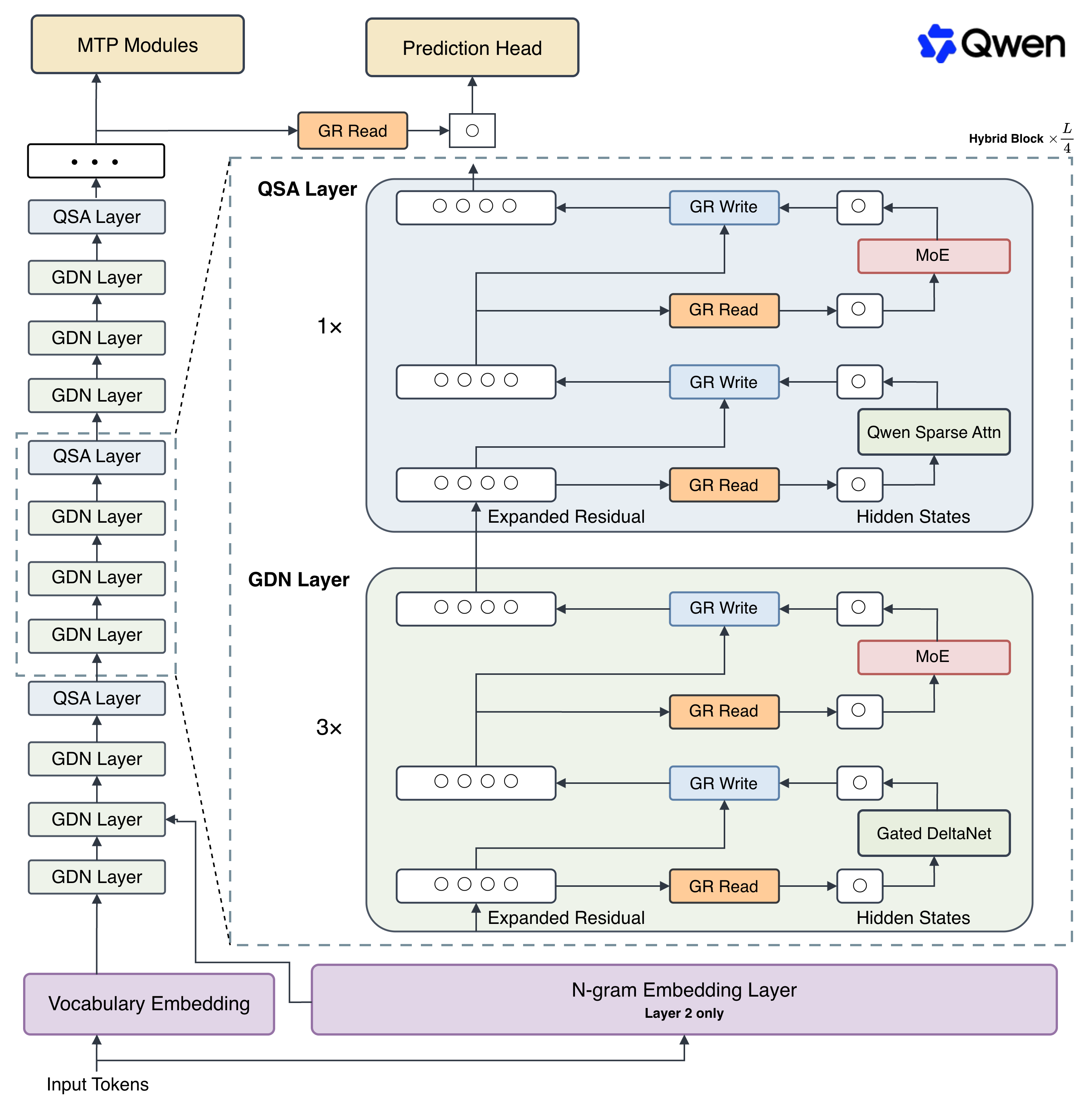
Token Embedding
  → 复制为 4 条 Residual Stream
  → 12 × [3 × (GDN → MoE) → 1 × (QSA → MoE)]
       每个子模块：Gated Read → Module → Gated Write
       第 2 层：额外注入 N-gram Embedding
  → Gated Read 合并 4 条 Stream
  → LM Head

模型配置如下。参数量中的 125B 指语言模型主干，每个 token 激活约 6B；此外还有 51B N-gram Embedding 和 4B MTP 参数。

组件	Qwen3.8-Flash-Next 配置
主干	48 层，隐藏维度 2560，125B 参数、每 token 激活 6B
层布局	36 层 GDN，12 层 QSA
QSA	24 个 Query Head、2 个 KV Head，Head Dim 256
QSA Indexer	4 个 Query Head、1 个 Key Head，Head Dim 128；每 4 token 压缩为一个 Micro-block
MoE	512 个 Routed Expert，每 token 选择 10 个，另有 1 个 Shared Expert
Gated Residual	4 条分支，门控瓶颈维度 320
N-gram Embedding	第 2 层注入；Bigram、Trigram 各 8 个 Hash Head，共 51B 参数
上下文	原生 262,144 token，可通过 YaRN 扩展到 1,000,000 token

Qwen3.5 已经使用 3 × GDN + 1 × Full Attention 的混合结构；Qwen3.8-Flash-Next 的关键变化是将 Full Attention 替换为 QSA，并把单路残差改为四路门控残差，同时加入 N-gram Embedding。GDN 的递推原理见 Qwen3.5。

2. Qwen Sparse Attention

QSA 位于 12 个全局检索层中，替代 Qwen3.5 的 Full Attention。它没有让压缩后的 Block Key 直接生成输出，而是把一次 Attention 拆成两个阶段：轻量 Indexer 先找出相关的连续 token 块，Sparse Core Attention 再用完整的 Key 和 Value 读取这些 token。图左侧负责“找”，右侧负责“读”。

2.1 设计目标

设当前有 $L_q$ 个 Query、$L_{kv}$ 个历史 token。Full Attention 需要计算 $L_q\times L_{kv}$ 个位置对，并读取全部历史 KV；当上下文扩展到数十万 token 时，Attention 计算和 KV Cache 访存都会随 $L_{kv}$ 增长。

一种直接的稀疏方案是先用轻量 Indexer 给每个历史 token 打分，再选择 Top-k token。然而 Indexer 仍要扫描 $L_{kv}$ 个候选位置，长上下文下它本身也会成为显著开销。QSA 将候选粒度从 token 改为包含 $c=4$ 个连续 token 的 Micro-block：

$${\mathrm{Cost}}_{QSA}\approx O\left(L_q\frac{L_{kv}}{c}{H}_I{d}_I\right)+O\left(L_{q}KHd\right)$$

第一项是轻量 Indexer 扫描压缩 Block 的成本，第二项是主 Attention 读取选中 token 的成本。Qwen3.8-Flash-Next 中，Indexer 使用 $H_I=4$、$d_I=128$，主 Attention 使用 $H=24$、$d=256$，Token Budget 为 $K=2048$。Indexer 仍随上下文线性增长，但它扫描的候选数缩小为约 $L_{kv}/4$，投影也远窄于主 Attention；主 Attention 的读取范围则限制在约 2048 个 token。

2.2 图中数据流

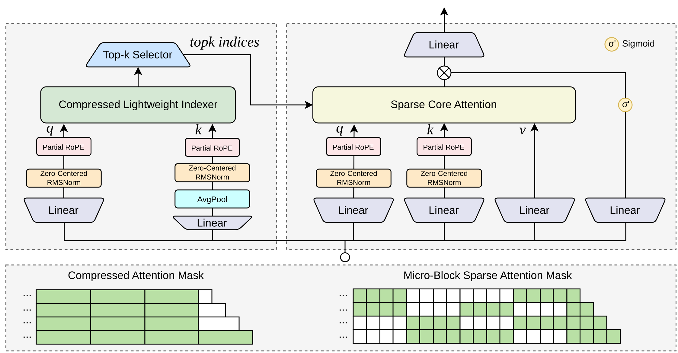
按照图中从下到上的数据流，QSA 完成以下步骤：

1. 两套投影：输入隐藏状态同时进入左侧 Indexer 和右侧主 Attention。两者有独立的 Query/Key 投影；Indexer 不计算 Value，因为它只负责选择位置。
2. Block 压缩：左侧 Key 路径先通过 Linear 得到逐 token Index Key，再由 AvgPool 把每 4 个连续 Key 平均为一个 Block Key。图底部的 Compressed Attention Mask 保证每个 Query 只能给因果范围内的完整 Block 打分。
3. Block 排序：Indexer Query 与全部可见 Block Key 计算相关性，Top-k Selector 为每个 Query 选择得分最高的 512 个 Block，并输出 topk indices。
4. Token 展开：每个选中 Block 重新展开为 4 个连续 token，因此 512 个 Block 对应最多 2048 个历史 token。图底部的 Micro-Block Sparse Attention Mask 中，绿色方格是主 Attention 保留的位置，白色方格不会参与读取。
5. 稀疏读取：右侧 Sparse Core Attention 使用主 Query、Key 和 Value，只在展开后的 token 集合上执行普通缩放点积注意力。
6. 输出门控：Attention 输出先与 Sigmoid 门逐元素相乘，再经过顶部 Linear 投影回隐藏维度。该门控制每个 Attention 输出特征写出多少信息，与 Indexer 的 Top-k 选择无关。

图中的 Zero-Centered RMSNorm 不表示对激活减均值。它仍只按均方根归一化，但缩放参数写为 $1+w$，并将 $w$ 初始化为 0，使归一化层初始缩放以 1 为中心。Partial RoPE 只旋转 Head 的前 64 维：对 128 维 Indexer Head 是一半维度，对 256 维主 Attention Head 是四分之一维度。

阶段	Query/Key 配置	候选范围	输出
Compressed Lightweight Indexer	4 个 Query Head、1 个 Key Head，Head Dim 128	约 $L_{kv}/4$ 个 Micro-block	每个 Query 的 512 个 Block ID
Sparse Core Attention	24 个 Query Head、2 个 KV Head，Head Dim 256	最多 2048 个选中 token，加不完整尾部	当前 Query 的 Attention 输出

2.3 Block 选择

设输入隐藏状态为 $X\in {\mathbb{R}}^{B\times L_q\times 2560}$。Indexer 的共享线性层将其投影并切分为：

$$Q^I\in {\mathbb{R}}^{B\times L_q\times 4\times 128},K^I\in {\mathbb{R}}^{B\times L_{kv}\times 128}$$

其中，历史 $K^I$ 会写入 Indexer Cache。对第 $j$ 个完整 Micro-block $G_j$，Transformers 参考实现先平均 4 个逐 token Key，再执行 RMSNorm 和 Partial RoPE：

$${\overline{k}}_j^I=\mathrm{RoPE}\left(\mathrm{RMSNorm}\left(\frac{1}{4}\sum _{i\in G_j}{k}_i^I\right)\right)$$

每个 Query 的 4 个 Indexer Head 分别与 Block Key 做点积。实现将负相关截断为 0，再对 Head 求和：

$$s_{t,j}=\frac{1}{\sqrt{128}}\sum _{h=1}^4\mathrm{ReLU}\left(⟨q_{t,h}^I,{\overline{k}}_j^I⟩\right)$$

Indexer 只需要对 Block 排序，因此无需对 $s_{t,j}$ 做 Softmax。选中的 Block 集合与主 Attention 的 token 集合分别为：

$${\mathcal{B}}_t=\mathrm{TopK}(s_t,min(512,N_t))$$$${\mathcal{S}}_t=\bigcup _{j\in {\mathcal{B}}_t}{G}_j\cup {\mathrm{CausalTail}}_t$$

其中，$N_t$ 是位置 $t$ 可见的完整 Block 数。CausalTail 是因果前缀末尾不足 4 个 token 的部分，它不参与平均和 Top-k，而是始终保留。这样既不会用未来 token 补齐 Block，也不会因为当前 Block 尚未完整而丢掉距离 Query 最近的 token。实现为每个 Query 预留 2048 + 4 - 1 = 2051 个索引槽位。

📄 Transformers：QSA Micro-block Indexer

class Qwen4ExpTextQSAIndexer(nn.Module):
    def __init__(self, config, layer_idx):
        ...
        self.token_budget = config.indexer_budget
        self.compress_ratio = config.indexer_compress_ratio
        self.block_topk = self.token_budget // self.compress_ratio

    def forward(self, hidden_states, position_embeddings, attention_mask, past_key_values):
        ...
        block_token_indices = local_visible_indices[
            : num_complete_blocks * self.compress_ratio
        ].view(num_complete_blocks, self.compress_ratio)
        key_groups = raw_keys[batch_idx].index_select(
            0, block_token_indices.flatten()
        ).view(*block_token_indices.shape, self.index_head_dim)
        pooled_keys = key_groups.float().mean(dim=1).to(raw_keys.dtype)
        pooled_keys = self.k_layernorm(pooled_keys)
        ...

        scores = torch.matmul(
            q[batch_idx, query_idx].float(),
            block_key_states.float().transpose(-1, -2),
        ).transpose(-1, -2)
        scores = torch.relu(scores).sum(dim=-1) / math.sqrt(self.index_head_dim)
        selected_block_indices = scores.topk(
            min(self.block_topk, num_complete_blocks), dim=0
        ).indices
        selected_tokens = block_token_indices.index_select(
            0, selected_block_indices
        ).flatten()
        ...
        tail = local_visible_indices[num_complete_blocks * self.compress_ratio :]
        selected_tokens = torch.cat([selected_tokens, tail])
        ...

2.4 稀疏主 Attention

Indexer 返回的 token 集合 ${\mathcal{S}}_t$ 会被转换为形状 [B, 1, L_q, L_{kv}] 的布尔或加性掩码，并与原始因果掩码合并。主 Attention 的张量为：

$$Q\in {\mathbb{R}}^{B\times 24\times L_q\times 256},K,V\in {\mathbb{R}}^{B\times 2\times L_{kv}\times 256}$$

这是 GQA：每个 KV Head 由 12 个 Query Head 共享。对 Query 位置 $t$，主 Attention 只在 $i\in {\mathcal{S}}_t$ 上归一化和聚合：

$$p_{t,h,i}=\frac{\exp \left(q_{t,h}^{\mathsf{T}}{k}_i/\sqrt{256}\right)}{\sum _{r\in {\mathcal{S}}_t}\exp \left(q_{t,h}^{\mathsf{T}}{k}_r/\sqrt{256}\right)},i\in {\mathcal{S}}_t$$$$o_{t,h}=\sum _{i\in {\mathcal{S}}_t}{p}_{t,h,i}{v}_i$$

因此，Block Key 只参与位置检索，不会替代主 Key；平均池化也不会作用于 Value。QSA 最终读取的是选中 Block 内每个 token 的完整 KV，这使模型既能降低读取范围，又保留 Block 内的 token 级细节。

主 Query 投影还同时产生一个与 Attention 输出等宽的门 $g_t$。24 个 Head 的输出拼接后先执行逐元素门控，再映射回 2560 维隐藏状态：

$$y_t=W_O(\mathrm{Concat}(o_{t,1},\dots ,o_{t,24})\odot \sigma (g_t))$$

📄 Transformers：Indexer 掩码与主 Attention

class Qwen4ExpTextAttention(Qwen3_5Attention):
    def forward(
        self,
        hidden_states,
        position_embeddings,
        attention_mask,
        past_key_values=None,
        **kwargs,
    ):
        selected_token_mask = self.indexer(
            hidden_states,
            position_embeddings,
            attention_mask,
            past_key_values,
        )
        if attention_mask.is_floating_point():
            attention_mask = attention_mask + selected_token_mask
        else:
            attention_mask = attention_mask & selected_token_mask

        position_embeddings = (
            x[:, -hidden_states.shape[1] :, :] for x in position_embeddings
        )
        return super().forward(
            hidden_states=hidden_states,
            position_embeddings=position_embeddings,
            attention_mask=attention_mask,
            past_key_values=past_key_values,
            **kwargs,
        )

📄 Transformers：主 GQA 与 Output Gate

class Qwen3NextAttention(Qwen3MoeAttention):
    def forward(self, hidden_states, position_embeddings, attention_mask, past_key_values=None, **kwargs):
        ...
        query_states, gate = torch.chunk(
            self.q_proj(hidden_states).view(*input_shape, -1, self.head_dim * 2),
            2,
            dim=-1,
        )
        gate = gate.reshape(*input_shape, -1)

        query_states = self.q_norm(query_states.view(hidden_shape)).transpose(1, 2)
        key_states = self.k_norm(
            self.k_proj(hidden_states).view(hidden_shape)
        ).transpose(1, 2)
        value_states = self.v_proj(hidden_states).view(hidden_shape).transpose(1, 2)

        cos, sin = position_embeddings
        query_states, key_states = apply_rotary_pos_emb(query_states, key_states, cos, sin)
        ...
        attn_output, attn_weights = attention_interface(
            self,
            query_states,
            key_states,
            value_states,
            attention_mask,
            scaling=self.scaling,
            **kwargs,
        )
        attn_output = attn_output.reshape(*input_shape, -1).contiguous()
        attn_output = attn_output * torch.sigmoid(gate)

        attn_output = self.o_proj(attn_output)
        return attn_output, attn_weights

2.5 Prefill 与 Decode

Prefill 和 Decode 使用同一套选择语义，但执行形态不同：

阶段	Query 数量	Block 选择	主 Attention
Prefill	Prompt 中的多个位置	每个 Query 根据自身因果前缀独立选择 Block，形成图中逐行不同的稀疏模式	Block-sparse Kernel 并行处理多个 Query 与各自选中的 KV
Decode	每步 1 个新 Query	扫描历史 Block Key，为当前 token 选择 512 个 Block	从 KV Cache 收集最多约 2048 个 token 的 KV，再生成一个输出

Decode 时，Indexer Cache 和主 KV Cache 都会追加当前 token。主 Attention 的读取预算不随上下文继续增大，但 Indexer 仍需扫描约 $L_{kv}/4$ 个 Block，因此总成本不是严格的常数。Prefill 时，每个 Query 的 Top-k 结果可能不同；高性能实现需要直接消费 Block ID 并执行块稀疏计算，而不是先构造完整的稠密 Attention 矩阵。

2.6 推理开销

36 个 GDN 层只维护固定大小的递推状态，随序列增长的 KV Cache 主要集中在 12 个 QSA 层。QSA 将每个 Query 的主 Attention 读取范围限制在选中的 Micro-block 内，因而减少长上下文计算和 KV 访存；连续选择 4-token Block 也比离散 token 索引具有更好的内存局部性。

QSA 不会消除 KV Cache。Indexer 需要保存历史 Index Key，12 个 QSA 层也要保存可被检索的完整主 KV；它减少的是每次参与主 Attention 的历史 token 数。当历史不超过约 2048 个 token 时，Top-k 会选中全部完整 Block，此时主 Attention 在语义上接近 Dense Attention，主要多出 Indexer 开销。

Transformers v5.16.1 参考实现逐 Query 使用 Python 循环选择 Block，再把结果转换为普通 Attention Mask，适合说明模型语义和验证正确性。官方性能数据依赖能根据 Block ID 收集 KV 并执行 Sparse Core Attention 的生产 Kernel，不能用该参考路径的吞吐直接代表 QSA 的硬件效率。

3. Gated Residual

标准 Transformer 让所有层读写同一条残差流。Gated Residual 将隐藏状态扩展为 $M=4$ 条并行分支，使每个 Attention/GDN 和 MoE 子模块都能动态决定从各分支读取哪些特征，以及将输出写回哪些分支。

设四分支状态为 $H\in {\mathbb{R}}^{B\times L\times M\times D}$。先对每条分支做 RMSNorm，再通过秩为 320 的瓶颈生成逐元素读门：

$$A=\sigma \left(W_{up}\mathrm{SiLU}(W_{down}\mathrm{vec}(\hat{H})/M)\right)$$$$x=\frac{1}{M}\sum _{m=1}^M{A}_m\odot {\hat{H}}_m$$

其中，$x\in {\mathbb{R}}^{B\times L\times D}$ 是当前子模块的输入。子模块输出 $F(x)$ 后，另一个门为每条分支产生一个写入系数：

$$g=2\sigma (W_g\mathrm{vec}(\hat{H})/M),H_m^{\prime }=H_m+g_{m}F(x)$$

读门细化到每个隐藏特征，写门则是每个 token、每条分支一个标量。模型入口将普通 Token Embedding 复制为四条流，末尾只执行门控读取，将四条流重新合并为一个隐藏状态。

📄 Transformers：Gated Residual 读写门

class Qwen4ExpTextGatedResidual(nn.Module):
    def forward(self, hyper_input):
        hyper_input_normed = self.hc_norm(hyper_input)
        input_mix_weight = F.silu(
            self.input_mix_weight_down(hyper_input_normed) / self.hc_count
        )
        input_mix_weight = torch.sigmoid(self.input_mix_weight_up(input_mix_weight))
        input_mix_weight = input_mix_weight.unflatten(
            -1, (self.hc_count, self.hidden_size)
        )
        mixed_input = (
            input_mix_weight
            * hyper_input_normed.unflatten(-1, (self.hc_count, self.hidden_size))
        ).mean(dim=-2)

        injection_weights = 2 * torch.sigmoid(
            self.block_inject_weight(hyper_input_normed) / self.hc_count
        )
        return mixed_input, hyper_input, injection_weights

四分支残差增加了残差激活和门控投影，但不把 Attention 或 Expert 的主计算扩展为四份。其目标是在较小额外计算下增加跨层信息路径，并降低深层网络反复混合导致的早期特征稀释。

4. N-gram Embedding

N-gram Embedding 根据当前 token 及其局部前缀直接查表，将模型容量从计算密集的矩阵乘法转移到内存访问。Qwen3.8-Flash-Next 在第 2 个 Decoder Layer 使用一层 N-gram Embedding，分别为 Bigram 和 Trigram 配置 8 个 Hash Head。

对长度为 $n$ 的局部 token 序列，第 $r$ 个 Hash Head 使用不同的奇数乘子 $p_i$ 和质数表大小 $V_{n,r}$ 计算索引：

$$h_{n,r,t}=\left(\underset{i=0}{\overset{n-1}{⨁}}{p}_i{\text{token}}_{t-i}\right)mod{V}_{n,r},n\in \{2,3\}$$

16 个 Head 的查表结果拼接为 2560 维向量。每个 Head 约有 2000 万个槽位、宽度为 160，合计约 51.2B 参数。随后 PLE 层根据 N-gram 特征和四条残差流计算注入门，并通过带膨胀率的 Depthwise Conv1d 补充局部组合信息。

📄 Transformers：N-gram Hash 与查表

class Qwen4ExpTextNGramEmbedding(nn.Module):
    def forward(self, input_ids, past_key_values):
        ...
        shifted_tokens = [
            self._shift_right_ignore_eos(token_history, shift)
            for shift in range(self.ngram_size)
        ]

        blocks = []
        for ngram in range(2, self.ngram_size + 1):
            start_idx = (ngram - 2) * self.heads_per_ngram
            end_idx = start_idx + self.heads_per_ngram
            mixed_ids = shifted_tokens[0] * self.layer_multipliers[0]
            for position in range(1, ngram):
                mixed_ids = torch.bitwise_xor(
                    mixed_ids,
                    shifted_tokens[position] * self.layer_multipliers[position],
                )
            head_vocab_sizes = self.ngram_heads_vocab_sizes[start_idx:end_idx]
            head_offsets = self.ngram_heads_offsets[start_idx:end_idx]
            ngram_ids = torch.remainder(
                mixed_ids.unsqueeze(-1), head_vocab_sizes.view(1, 1, -1)
            )
            blocks.append(ngram_ids + head_offsets.view(1, 1, -1))

        ngram_ids = torch.cat(blocks, dim=-1)[:, -input_ids.shape[1] :]
        return self.ngram_embedding(
            ngram_ids.to(self.ngram_embedding.weight.device)
        ).to(ngram_ids.device).flatten(-2)

查表位置可由 token ID 提前确定，因此官方设计允许把这 51B 参数放在 Host Memory，并用异步预取与模型计算重叠。这并不消除内存成本：实际收益取决于主机内存容量、CPU–GPU 带宽、预取实现和尾延迟；普通框架中的同步设备拷贝也不自动具备该重叠能力。

5. MoE、MTP 与训练优化

每个 Decoder Layer 包含 512 个 Routed Expert，Router 为每个 token 选择 10 个，并始终执行 1 个 Shared Expert；每个 Expert 的中间维度为 640。大专家池提高总容量，而固定的激活专家数将每 token 参与计算的主干参数控制在约 6B。

模型还包含一个约 4B 参数的单层 Multi-Token Prediction（MTP）模块，并对多个未来步联合训练。MTP 可改善主干训练，也可作为自投机解码的 Draft；Qwen3.8-Flash-Next 的 MTP Attention 同样使用 QSA。

训练侧使用 Muon 与 AdamW 分工：Attention、GDN 和 MoE Expert 等二维线性映射使用 Muon，Embedding、MoE Router 与 Gated Residual 的低秩参数使用 AdamW；融合的 QKV、SwiGLU 和 GDN 投影会先按独立线性映射拆分，再分别正交化。官方实验据此重新拟合 Scaling Law，并取消 Batch Size Warmup；在其对照中，Warmup 没有改善最终结果，却多消耗 18.8% 的优化器步数。

6. 性能与边界

官方博客在 1M token 上下文下报告，QSA Attention Kernel 的 Prefill 与 Decode 最高分别加速 7.6 倍和 4.9 倍。在 90% Prefix Cache 命中率的在线服务实验中，Qwen3.8-Flash-Next 的 1M 上下文 Prefill 吞吐为 Qwen3.7-Plus 的 8.6 倍。

这些数字是特定 Kernel、上下文长度和缓存命中率下的结果，不能直接外推到短请求、Transformers 参考实现或其他硬件。模型的推理成本还受 512 Expert 的权重驻留、51B N-gram 表的放置方式、QSA 索引器开销和四分支残差激活影响；“每 token 激活 6B”描述计算稀疏性，不代表部署时只需存放 6B 参数。

7. 参考

1. Qwen：Qwen3.8-Flash-Next 官方博客
2. Qwen：Qwen3.8-Flash-Next 技术报告
3. Hugging Face：Qwen3.8-Flash-Next 模型卡
4. Hugging Face：Qwen3.8-Flash-Next 配置
5. Transformers：Qwen4 Experimental 参考实现（v5.16.1）